Biosimilarity on survival endpoints: a relative-distance test for three-arm trials with two reference products
How to judge a biosimilar on a survival endpoint by measuring its distance from two licensed versions of the reference product in units of the distance between those two versions, and three ways to estimate that ratio, from a constant-hazard model to one that needs no proportional hazards at all.
Biosimilars are follow-on versions of licensed biologic medicines, and before one is approved it has to show in a clinical trial that it performs like the original. The standard phase III design has two arms, biosimilar against reference, and asks whether the absolute difference between them stays inside a fixed margin. What that design leaves out is that the reference product is not a single fixed thing either. Biologics are heterogeneous by nature and often highly variable, so the same medicine licensed in the EU and in the US can differ slightly, and a margin that ignores this variability can be too strict or too loose for reasons that have nothing to do with the biosimilar.
Kang and Chow proposed an alternative for continuous endpoints in 2013: randomise patients to the biosimilar and to two licensed versions of the reference, and judge the biosimilar's distance from the reference against the distance between the two references. Shin and Kang later extended it to binary endpoints. This article, my first-author methodology paper and the core of my Ph.D. dissertation, extends the design to time-to-event endpoints, where censoring and the shape of the hazard over time make the problem harder. The test is worked out three times, under an exponential model, under the Cox proportional hazards model and with the restricted mean survival time (RMST), each with an asymptotic test, a power function and a sample-size method, and every version is checked by simulation.
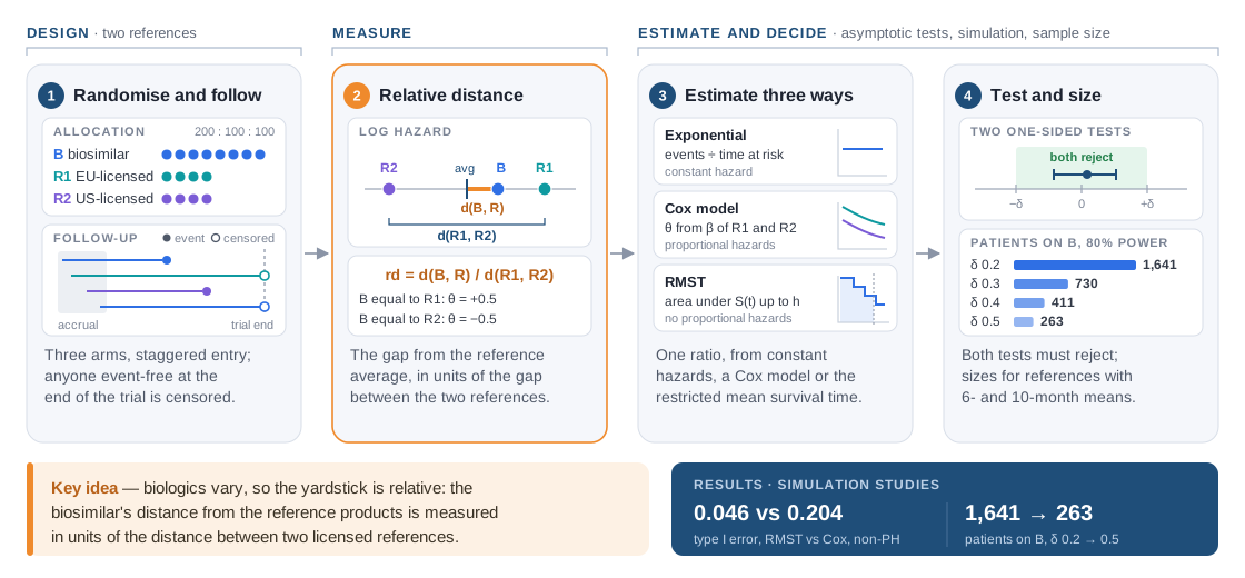
The simulations separate the three versions clearly. The exponential and Cox tests kept the type I error close to the nominal 5% when their assumptions held. When the Weibull shape parameters of the three arms differed only slightly, 1.0, 0.95 and 1.05, the Cox-based test claimed biosimilarity far too often, 0.204 in one setting where the RMST-based test stayed at 0.046. Wider margins need far fewer patients: with reference means of 6 and 10 months, the biosimilar arm needs 1,641 patients for 80% power at a margin of 0.2 and 263 at 0.5. I developed the asymptotic testing procedures, the simulation-based validation and the sample-size methods. This post walks through the design, the margin, the three estimators and what the simulations say about choosing between them.
Two reference products as the yardstick
Label the biosimilar B, the EU-licensed reference R1 and the US-licensed reference R2. Patients are randomised 2:1:1, so the biosimilar arm is as large as the two reference arms together. That allocation answers the obvious objection that a third arm costs 50% more patients: a two-arm trial with 200 patients per arm and a three-arm trial with 200 on the biosimilar and 100 on each reference both enrol 400.
For a survival endpoint, distance is measured on the log-hazard scale. The location of "the reference" is the average of the two reference log hazards. The relative distance is the absolute difference between the biosimilar's log hazard and that average, divided by the absolute difference between the two reference log hazards. Writing the signed version of the ratio as θ, the question becomes an equivalence problem: the null hypothesis says θ is at most −δ or at least +δ, the alternative says θ lies strictly between, for a margin δ fixed in advance.
The ratio has a concrete reading. If the biosimilar's hazard equals R1's, θ is +0.5; if it equals R2's, θ is −0.5; anywhere between the two references, its absolute value is below 0.5. A margin around 0.5 therefore asks for a biosimilar that sits no further from the reference average than the licensed products themselves do, which is why the type I error simulations concentrate on margins of 0.4, 0.5 and 0.6.
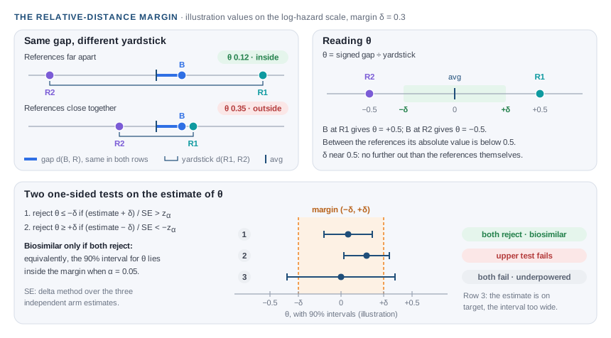
The equivalence null is the union of two one-sided nulls, so the test is a pair of one-sided tests. The first rejects θ at most −δ when the estimate plus δ, divided by its standard error, exceeds the upper α quantile of the normal distribution; the second rejects θ at least +δ when the estimate minus δ, divided by its standard error, falls below the negative of that quantile. Biosimilarity is claimed only if both reject at level α. The standard error comes from the delta method: the three arms are independent, each arm's estimate is asymptotically normal, and θ is a smooth function of them. Natural uses are bridging a foreign-licensed reference product with clinical rather than pharmacokinetic endpoints, and multi-regional programmes that already compare a biosimilar with both references.
One ratio, three ways to estimate it
What changes across the three versions is how each arm's survival is summarised and how much the model assumes about it.
Exponential model. With a constant hazard, the maximum likelihood estimate of each arm's hazard is the number of events divided by the total follow-up time. Following Lachin and Foulkes, patients enter during an accrual period with entry times from a truncated exponential distribution, uniform as a special case, and everyone still event-free when the trial closes is censored. The asymptotic variance of each log hazard then has a closed form in the accrual length, the total trial length and the entry pattern, so the test, its power and the sample size can be written down directly. It is the cleanest setting for the idea, at the price of a strong assumption.
Cox proportional hazards model. Two indicator variables mark R1 and R2, with the biosimilar as the baseline group, and covariates such as age or disease severity can be added. The hazard ratio of the biosimilar against R1 is the exponential of minus the first coefficient, and θ becomes a function of the two arm coefficients alone, with its variance from the inverse information matrix and the delta method. The baseline hazard is left unspecified, which suits real survival curves, but the arms must have proportional hazards; the article suggests log-minus-log Kaplan–Meier plots or a goodness-of-fit test as checks. For sample size, the information depends on the number of deaths, not patients. The method finds the minimum total number of deaths, approximating the information with Luo and Su's ten-quantile approach under Weibull distributions with a common shape, then converts deaths into patients through each arm's event probability by the end of follow-up.
Restricted mean survival time. RMST up to a horizon h is the area under the survival curve from zero to h, the expected event-free time within the window, and it needs no proportional hazards. Each patient gets a pseudo-observation, the jackknife contrast between the Kaplan–Meier estimate of RMST with and without that patient, so censored patients still carry information. Regressing the pseudo-observations on the three arm indicators with an identity link and generalised estimating equations returns the three arm means and a sandwich variance, and θ is built from RMST differences instead of log hazards. Unlike the hazard-based ratio, this one depends on the horizon, which the simulations had to account for when comparing versions.
Results
Empirical type I error at the margin boundary, with 200 to 1,000 patients on the biosimilar and follow-up to 12 or 24 months (nominal level 0.05; 5,000 replications per setting for the exponential and Cox versions):
| Version | Simulated survival times | Type I error range |
|---|---|---|
| Exponential model | constant hazards | 0.023–0.057 |
| Cox model | Weibull, equal shapes (proportional hazards) | 0.022–0.082 |
| Cox model | Weibull, shapes 1.0, 0.95, 1.05 | 0.102–0.838 |
| RMST | Weibull, equal shapes | 0.022–0.082 |
| RMST | Weibull, shapes 1.0, 0.95, 1.05 | 0.022–0.075 |
The Cox inflation is not a small-sample artefact. In the first setting it rose from 0.204 with 200 patients on the biosimilar to 0.480 with 1,000, the signature of bias rather than noise: a misspecified hazard ratio is estimated ever more precisely around the wrong value. RMST held its level in the same settings. For sizing, theoretical and simulated power agreed reasonably well. With reference means of 6 and 10 months, a 12-month trial and 80% target power, the exponential test needs 1,641 patients on the biosimilar at δ = 0.2, 730 at 0.3, 411 at 0.4 and 263 at 0.5, with simulated powers between 0.75 and 0.81. The RMST version tended to need fewer patients than the Cox version, for example 802 against 934 in the same setting at a base margin of 0.3, although the article notes the two cannot be compared exactly. The methods ship with the article as the R package Biosimilar3ArmSurv.
What I learned
Calibrate a margin by the variability you cannot remove. An absolute margin has to be argued from outside the trial. A relative margin borrows its scale from inside it: the observed difference between two licensed versions of the same product is exactly the amount of variation a patient or regulator already accepts.
An equivalence test is only as honest as its model. A five per cent difference in Weibull shape is invisible on a survival plot, yet it pushed the Cox version's type I error to between two and seventeen times the nominal level, worse with every added patient. Choosing the RMST version when proportional hazards are doubtful is a design decision, not a detail of analysis.
In survival trials, information is counted in events. The Cox sample size is really a number of deaths, and the follow-up time and event rate decide how many patients it takes to observe them. Writing the power function in terms of events made it obvious where a trial gains or loses precision.
Limitations
- The design assumes no between-batch variability within each product; incorporating batches would make the design more complex and is left for future work.
- There is no settled way to choose the margin for time-to-event endpoints; margin proposals so far cover continuous endpoints.
- The ratio becomes unstable when the two reference products are nearly identical, because its denominator approaches zero; a modified procedure exists for continuous endpoints but has not yet been adapted to survival data.
All numbers come from the published article and the dissertation, and every result is from simulation, so no patient data are involved. The figures are drawn for this site; values marked as illustration are invented to explain the method.